
MNIST style digit example - 28×28 grayscale, handwritten
The MNIST database is one of the most well known in the ML world, and for good reason. 70,000 28x28px, hand-drawn, and human-labeled numbers in greyscale on a black backdrop? The embodiment of consistency and perfect for an introduction to neural nets.
This post will serve as a bit of a stream-of-consciousness to organize my observations and learnings getting my hands dirty building my first neural network. No more theory, let’s build and tweak it to see first hand the impacts of optimizers, hidden layer count/size, learning rate, and anything else we find along the way.
The Setup
I first initialized my dataset (provided conveniently through torchvision) by transforming to tensor and normalizing with MNIST’s provided mean (0.1307) and STD (0.3081). Prepped the 10k test data set and the 60k training images, set my batch to 64 for speed and smoother gradient estimates, and ensured the data was shuffled so I wasn’t training on the order.
I set up my Multilayer Perceptron to have two hidden layers of 128 and 64 neurons sandwiched by a layer of 784 inputs and a layer of 10 outputs. The 10 output logits of course corresponding to the ‘predicted’ output digit.
flattened 784 inputs -> 128 hidden -> 64 hidden -> 10 outputs
PyTorch’s CrossEntropyLoss() function exists to take care of Softmax’ing and calculating loss. I first went with Adaptive Moment Estimation with a learning rate of 1e-3 for the optimizer, but left myself a little commented line as a treat for later to swap to Stochastic Gradient Descent at lr=0.01. I knew I was going to want to swap them and witness the difference.
I also created a matching Convolutional Neural Network to swap in and compare to the MLP later. I set the CNN up with a 3x3 kernel, 2 conv layers bringing the filters from 1 input channel->32->64 feature maps, and a single ‘pixel’ of padding per layer to maintain dimensions. Sequentially MaxPool2d() downsampled each map down per layer to half the dimensions (final 7x7 down from 28 x 28) for speed and position tolerance (handwriting is far from precise, so this makes particular sense to use here). The final connection back to the expected 10 output logits is a flattening of the 64, 7x7 maps to 3136->128->10
Lastly my eval method would check how many correct over the total and output a convenient accuracy %. Later I realized it was crucial to see the state of the nn before training for comparison, and made an Epoch 0 accuracy check before training. But till then I strictly checked accuracy post training.
Full training script — click to expand mnist_train.py
import torch
from torchvision import datasets, transforms
from torch.utils.data import DataLoader, random_split
import torch.nn as nn
import torch.nn.functional as F

transform = transforms.Compose([
    transforms.ToTensor(),                       # image -> tensor, scales pixels to [0.0, 1.0]
    transforms.Normalize((0.1307,), (0.3081,)),  # subtract mean, divide by std (MNIST's known stats)
])

train_data = datasets.MNIST(root="./data", train=True,  download=True, transform=transform)
test_data  = datasets.MNIST(root="./data", train=False, download=True, transform=transform)

# pre select 10% of the training set for validation
train_subset, val_subset = random_split(
    train_data, [54000, 6000],
    generator=torch.Generator().manual_seed(19) #set the seed to ensure selected data remains constant
)

#Dataloader handles the batch grouping,shuffling, and iteration
train_loader = DataLoader(train_subset, batch_size=64, shuffle=True)
val_loader   = DataLoader(val_subset,   batch_size=1000, shuffle=False)
test_loader  = DataLoader(test_data,  batch_size=1000, shuffle=False)

images, labels = next(iter(train_loader))

#Build the MLP
class MLP(nn.Module):
    def __init__(self):
        super().__init__()
        self.fc1 = nn.Linear(28 * 28, 128)   # 784 inputs -> 128 hidden
        self.fc2 = nn.Linear(128, 64)        # 128 -> 64 hidden
        self.fc3 = nn.Linear(64, 10)         # 16 -> 10 logits output (one per digit)

    def forward(self, x):
        x = x.view(x.size(0), -1)   # flatten [64, 1, 28, 28] -> [64, 784]
        x = F.relu(self.fc1(x))     # layer 1 + activation
        x = F.relu(self.fc2(x))     # layer 2 + activation
        x = self.fc3(x)             # output logits
        return x

#Build a CNN for comparison to MLP
class CNN(nn.Module):
    def __init__(self):
        super().__init__()
        self.conv1 = nn.Conv2d(1, 32, kernel_size=3, padding=1)   # 1 channel in, 32 feature maps out
        self.conv2 = nn.Conv2d(32, 64, kernel_size=3, padding=1)  # 32 -> 64 feature maps
        self.pool  = nn.MaxPool2d(2, 2)                           # halves height & width
        self.fc1   = nn.Linear(64 * 7 * 7, 128)
        self.fc2   = nn.Linear(128, 10)
        self.dropout = nn.Dropout(0.25)

    def forward(self, x):
        x = self.pool(F.relu(self.conv1(x)))   # [B,1,28,28] -> [B,32,14,14]
        x = self.pool(F.relu(self.conv2(x)))   # [B,32,14,14] -> [B,64,7,7]
        x = x.view(x.size(0), -1)              # flatten -> [B, 64*7*7 = 3136]
        x = F.relu(self.fc1(x))
        x = self.dropout(x)                    # randomly zero 25% of activations (regularization)
        x = self.fc2(x)
        return x

#method for evals
def evaluate(model, loader):
    model.eval()                       # eval mode (disables dropout, etc)
    correct = total = 0
    with torch.no_grad():              # disable building the autograd graph for eval
        for images, labels in loader:
            images, labels = images.to(device), labels.to(device)
            outputs = model(images)
            predicted = outputs.argmax(dim=1)   # index of highest logit = predicted digit
            correct += (predicted == labels).sum().item()
            total += labels.size(0)
    return 100 * correct / total

#Loss and optimizer
device = torch.device("cuda" if torch.cuda.is_available() else "cpu")
model = MLP().to(device)

criterion = nn.CrossEntropyLoss()
optimizer = torch.optim.Adam(model.parameters(), lr=1e-3) #try Adam (most efficient)
#optimizer = torch.optim.SGD(model.parameters(), lr=0.01, momentum=0.9) #try Stochastic Gradient Descent
epochs = 5

val_acc = evaluate(model, val_loader)
print(f"Epoch 0  val acc {val_acc:.2f}%")   #view accuracy before training

for epoch in range(epochs):
    model.train()
    running_loss = 0.0

    for images, labels in train_loader:
        images, labels = images.to(device), labels.to(device)

        optimizer.zero_grad()               # 1. clear old gradients
        outputs = model(images)             # 2. forward pass -> logits
        loss = criterion(outputs, labels)   # 3. how wrong is the prediction?
        loss.backward()                     # 4. backprop: compute gradients
        optimizer.step()                    # 5. nudge weights downhill

        running_loss += loss.item()
    val_acc = evaluate(model, val_loader)
    print(f"Epoch {epoch+1}: loss {running_loss/len(train_loader):.4f}  val acc {val_acc:.2f}%")

#torch.save(model.state_dict(), "mnist.pt")     #uncomment to save the final state to load later

print(f"Test accuracy: {evaluate(model, test_loader):.2f}%")
I set up my training loop with the core 5 step forward pass to back propagation cycle:
optimizer.zero_grad()               # 1. clear old gradients
outputs = model(images)             # 2. forward pass -> logits
loss = criterion(outputs, labels)   # 3. how wrong is the prediction?
loss.backward()                     # 4. backprop: compute gradients
optimizer.step()                    # 5. nudge weights downhill
First training run, 5 epochs
My first training run, 5 epochs
Epoch 1: avg loss 0.2723
Epoch 2: avg loss 0.1177
Epoch 3: avg loss 0.0798
Epoch 4: avg loss 0.0613
Epoch 5: avg loss 0.0503
Test accuracy: 97.41%
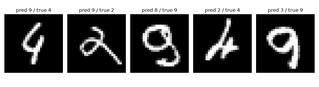
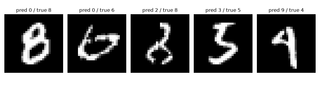
MLP, Adam. A loss reduction of 0.2220 over 5 epochs resulting in a neural net able to correctly discern 97.41% of the digits from the images in the withheld test set. Absolutely incredible. After a few runs, looking at a selection of the digits it would get wrong: the majority of them are completely understandable:
Lets get tweakin.
What I assumed would be the biggest factor: more epochs!
More epochs means more passes iterating over the data and updating weights. My theory is that the more epochs, the lower the loss and the higher the accuracy until the dreaded ‘overfit’ wall is reached. That matched pretty well with what I saw. Adding more epochs marginally increased accuracy until a point where the accuracy started to drop. It also was the only knob turned that meaningfully increased training time.
| 5 Epochs | 6 Epochs | 10 Epochs |
|---|---|---|
| Epoch 5: avg loss 0.0503 Test accuracy: 97.41% | Epoch 6: avg loss 0.0384 Test accuracy: 97.89% | Epoch 10: avg loss 0.0227 Test accuracy: 97.71% |
What ACTUALLY was the biggest factor: getting convolved
Turns out the most important detail was the model structure itself, who knew. The Convolutional Neural Net is substantially better suited to the task of image classification and it shows. The loss converged much quicker and the final accuracy over the test data was better than any result I was able to squeeze out of the MLP. This sent me on a tangent diving into convolution. Also of note, dropout. Zeroing out a percentage of activations per run in order to prevent the network from favoring specific activations too heavily. Reduce overfitting. Spicy stuff.
CNN 5 epochs
CNN 5 epochs
Epoch 1: avg loss 0.1623
Epoch 2: avg loss 0.0553
Epoch 3: avg loss 0.0402
Epoch 4: avg loss 0.0304
Epoch 5: avg loss 0.0250
Test accuracy: 99.26%
A swap to SGD
Even before going into this I had heard of Adam and fully expected it to outshine SGD, but was excited to actually see the behavioral differences. Up till this point I had stuck with the best-in-slot optimizer, but swapped to SGD to run similar tests and make some observations.
Initially I didn’t notice an obvious difference, but then I started cranking the epochs. It seems that SGD is either more resilient to overfitting or simply takes longer to reach it. Regardless it takes longer overall to reach an improved accuracy. The accuracy was getting better and loss lower even up through 20 epochs! But somewhere around 27 the loss would fall to 0.0000 and accuracy would plummet. I believe I’ve heard the term for this is ’explode’. This difference is probably due to the learning rate variance as Adam adapts its step size during training. A strict slow rate would take more epochs to converge.
| 5 Epochs | 10 Epochs | 20 Epochs | 40 Epochs |
|---|---|---|---|
| Epoch 5: avg loss 0.0465 Test accuracy: 97.61% | Epoch 10: avg loss 0.0124 Test accuracy: 97.90% | Epoch 20: avg loss 0.0005 Test accuracy: 98.25% | Epoch 40: avg loss 0.0000 Test accuracy: 98.00% |
Two more knobs: layers and neuron count
My last point of interest for tweaking was to modify both the number of hidden layers and the number of neurons in each.
- Adding layers - I first brought the network from
784->128->64->10to784->128->64->32->10then784->128->64->32->16->10. I saw no meaningful change in output. Accuracy began dropping before 10 epochs and before any notable gains. - More neurons -
784->256->128->10did result in a better accuracy and lower loss at epoch 5 than the reference MLP. Is bigger better?784->512->256->10said no, loss was lower but accuracy fell. - Combine them - More and More!
784->512->256->128->64->10- Nothing thrilling, behaved similarly to256->128->10and increasing epochs didn’t improve things past 5.
Improved, validation-added
After all my experiments I realized it would be useful to bake in a random split of some amount of the training data to validate against each epoch. This would allow me to get a glimpse into how accuracy is increasing (or decreasing) each pass. PyTorch has a built in support for this of course with random_split. Manual seed prevents every pass from getting a new random set. I also added a quick check prior to training to actually visualize the default state of the network. Seeing it genuinely go from a random 1/10 guess to 95%+ accuracy in one pass is incredible.
train_subset, val_subset = random_split(
    train_data, [54000, 6000],
    generator=torch.Generator().manual_seed(19)
)
Output
val add split
Epoch 0  val acc 10.27%
Epoch 1: loss 0.3296  val acc 95.40%
Epoch 2: loss 0.1160  val acc 97.48%
Epoch 3: loss 0.0789  val acc 98.07%
Epoch 4: loss 0.0575  val acc 97.82%
Epoch 5: loss 0.0458  val acc 98.93%
Test accuracy: 97.58%
It was interesting to see here that the val accuracy was actually higher than the final test accuracy and jumpy between epochs. This jumpiness reflects the increased sampling noise from a set that’s only 60% the size. It really highlights the importance of bigger evaluation sets. The more data, the less the results are at the mercy of noise.
It also seems to confirm a weakness in my entire experiment that I’ve had in the back of my mind: the margin for noise may exceed any observed accuracy changes. To be confident in the statistical significance of changes in accuracy, I would really need to execute many, many more training runs and average the results rather than letting my monkey brain cherry-pick the results that validate my bias.
Searching around a bit, it turns out the test-validation accuracy gap is actually explained by the pool of writers being different between the train and test sets. The net is trained on the 60k written by one set of writers (more precisely, 54k since 6k are held for val), and then evaluated on the 10k written by another. No writer appears in both sets. Handwriting differences would certainly explain a bit of the gap between val and final accuracy.
The final step, trying my own digits!
I added a line to save a checkpoint and created a loader to feed in some numbers I drew on a 28x28 image in Photoshop. This allowed me to see the fruits of my labor. The top 3 predictions and their confidence are included.
| Digit |  |  |  |  |
|---|---|---|---|---|
| Prediction | prediction: 2 (98.7% confident) 2 - 98.7% 8 - 0.3% 0 - 0.0% | prediction: 4 (96.5% confident) 4 - 96.5% 9 - 2.8% 1 - 0.2% | prediction: 5 (99.1% confident) 5 - 99.1% 9 - 0.8% 3 - 0.1% | prediction: 7 (69.3% confident) 7 - 69.3% 2 - 22.4% 3 - 6.6% |
My drawn 7 was definitely not up to MNIST standard (centered, properly padded, etc), but it predicted correctly. Pretty impressive!
Conclusion
I never trained on the test data, but made many decisions based on it. Unfortunately as a human I make an ineffective outer optimization loop as I'm far from immune to the effects of noise. In reality, the only concrete outcome was the improvement in accuracy for CNN over MLP. Most of the rest plays around the noise floor. Regardless, this project was a much needed step into the inner workings of neural nets and fuels my interest to continue.What else?
There are obviously far too many facets to tweak for a weekend project. At some point I'll revisit for further experimentation with how the following impact the results:- CNN: changing the number of conv layers, modifying pooling strategy, kernel dimension change.
- LR: controlled for model type, increase and decrease the learning rate.